Factorization

src: i.ytimg.com

In mathematics, factorization (also factorisation in some forms of British English) or factoring consists of writing a number or another mathematical object as a product of several factors. For example, 3 × 5 is a factorization of the integer 15, and (x - 2)(x + 2) is a factorization of the polynomial x² - 4.

Factorization is not usually considered for rational and real numbers, because, for every pair (x, y) of nonzero such numbers, there is a factorization x = y z, with z = x / y.

Factorization has been considered first by ancient Greek mathematicians, in the case of integers. They proved the fundamental theorem of arithmetic, which asserts that every positive integer may be factorized into a product of specific integers called prime numbers, that have the property of not having any factorization in factors different of one. Moreover, this factorization is unique up to the order of the factors. Factorization is, somehow, the inverse operation of multiplication. However, in the case of large integers, integer factorization is much more difficult than multiplication, and this is widely used in public-key cryptography, typically through the RSA cryptosystem.

Factorization is a useful tool for simplifying expressions and reducing the problem of solving an equation to solving several simpler equations. However, except for specific classes of expressions, such as polynomials, there is no general algorithm of factorization. There are only heuristic methods, which are often useful for paper-and-pencil computation on simple examples.

Polynomial factorization is also considered since a long time. Polynomials with integer coefficients or coefficients in a field have the unique factorization property, that is, they verify a theorem that is very similar to the fundamental theorem of arithmetic, with prime numbers replaced by irreducible polynomials. In particular, a univariate polynomial with complex coefficients, admits a unique (up to the order of the factors) factorization into linear polynomials; this is the fundamental theorem of algebra. In this case, the factorization is usually done with root-finding algorithms. The case of polynomials with integer coefficients is fundamental for computer algebra. There are algorithms for computing the (complete) factorization of any polynomial with integer coefficients (see factorization of polynomials); although they are very efficient for a computer usage, they are generally too complicate for being used in paper-and-pencil computation.

The commutative rings in which unique factorization property holds are called unique factorization domains. There are number systems which are not unique factorization domains. This is the case of many rings of algebraic integers. However, these are Dedekind domains, which means that unique factorization property holds if one replaces factorization into algebraic integers by factorization into ideals.

Factorization is often used for the decomposition of a mathematical object into the product of objects of a more specific type. For example every function may be factored into the composition of a surjective function with an injective function. For matrices, there are many kinds of such matrix factorizations. For example, every matrix has a LUP factorization as a product of a square lower triangular matrix L with all diagonal entries equal to one, an upper triangular matrix U, and a permutation matrix P.

Video Factorization

Integers

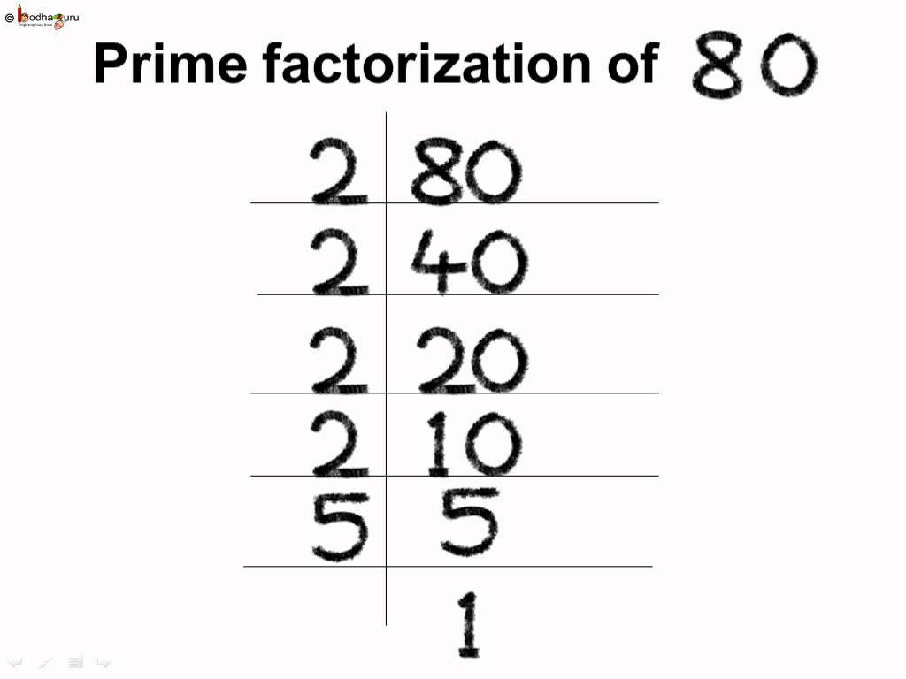
By the fundamental theorem of arithmetic, every integer greater than 1 has a unique (up to the order of the factors) factorization into prime numbers, which are those integers which cannot be further factorized into the product of integers greater than one.

For computing the factorization of an integer n, one needs an algorithm for finding a divisor q of n or deciding that n is prime. When such a divisor is found, the repeated application of this algorithm to the factors q and n / q gives eventually the complete factorization of n.

For finding a divisor q of n, if any, it suffices to test all values of q such that 1 < q and q² <= n. In fact, if r is a divisor of n such that r² > n, then q = n / r is a divisor of n such that q² <= n.

If one tests the values of q in increasing order, the first divisor that is found is necessarily a prime number, and the cofactor r = n / q cannot have any divisor smaller than q. For getting the complete factorization, it suffices thus to continue the algorithm by searching a divisor of r that is not smaller than q and not greater than ?r.

There is no need to test all values of q for applying the method. In principle, it suffices to test only prime divisors. This needs to have a table of prime numbers that may be generated for example with the sieve of Eratosthenes. As the method of factorization does essentially the same work as the sieve of Eratosthenes, it is generally more efficient to test for a divisor only those numbers for which it is not immediately clear whether they are prime or not. Typically, one may proceed by testing 2, 3, 5, and the numbers > 5, whose last digit is 1, 3, 7, 9 and the sum of digits is not a multiple of 3.

This method works well for factoring small integers, but is inefficient for larger integers. For example, Pierre de Fermat was unable to discover that the 6th Fermat number

${\displaystyle 1+2^{2^{5}}=1+2^{32}=4,295,967,297}$

is not a prime number. In fact, applying the above method would require more than 10,000 divisions, for a number that has 10 decimal digits.

There are more efficient factoring algorithms. However they remain relatively inefficient, as, with the present state of the art, one cannot factorize, even with the more powerful computers, a number of 500 decimal digits that is the product of two randomly chosen prime numbers. This insures the security of the RSA cryptosystem, which is widely used for secure communications on Internet.

Example

For factoring n = 1386 into primes:

• Start with division by 2: the number is even, and n = 2 · 693. Continue with 693, and 2 as a first divisor candidate.
• 693 is odd (2 is not a divisor), but is a multiple of 3: one has 693 = 3 · 231 and n = 2 · 3 · 231. Continue with 231, and 3 as a first divisor candidate.
• 231 is also a multiple of 3: one has 231 = 3 · 77, and thus n = 2 · 3² · 77. Continue with 77, and 3 as a first divisor candidate.
• 77 is not a multiple 3, since the sum of its digits is 14, not a multiple of 3. It is also not a multiple of 5 because its last digit is 7. The next odd divisor to be tested is 7. One has 77 = 7 · 11, and thus n = 2 · 3² · 7 · 11. This shows that 7 is prime (easy to test directly). Continue with 11, and 7 as a first divisor candidate.
• As 7² > 11, one has finished. Thus 11 is prime, and the prime factorization is

1386 = 2 · 3² · 7 · 11.

Maps Factorization

Expressions

Manipulating expressions is the basis of algebra. Factorization is one of the most important methods for expression manipulation for several reasons. If one can put an equation in a factored form E?F = 0, then the solving problem splits into two independent (and generally easier) problems E = 0 and F = 0. When an expression can be factored, the factors are often much simpler, and may, therefore, some insight on the problem. For example,

${\displaystyle x^{3}-ax^{2}-bx^{2}-cx^{2}+abx+acx+bcx-abc}$

may be factored into the much simpler expression (two multiplications and three additions instead of 16 multiplications, 4 subtractions and 3 additions)

${\displaystyle (x-a)(x-b)(x-c).}$

Moreover, the factored form gives immediately the roots of the polynomial in x represented by these expressions.

On the other hand, factorization is not always possible, and when it is possible, the factors are not always simpler. For example, ${\displaystyle x^{999}-1}$ can be factored into two irreducible factors, one of them having 1000 terms.

Various methods have been developed for finding factorizations; some are described below.

Solving algebraic equations may be viewed as a problem of factorization. In fact, the fundamental theorem of algebra can be stated as follows. Every polynomial in x of degree n with complex coefficients may be factorized into n linear factors ${\displaystyle x-a_{i},}$ for i = 1, ..., n, where the a_is are the roots of the polynomial. Even though the structure of the factorization is known in these cases, the a_is can generally not computed exactly, as the Abel-Ruffini theorem shows (roughly speaking) that the a_is coefficients can generally not be represented by an usual expression. Therefore, in most cases, the best that can be done is computing approximate values of the roots with a root-finding algorithm.

History of factorization of expressions

The systematic use of algebraic manipulations for simplifying expressions (more specifically equations)) may be dated to 9th century, with al-Khwarizmi's book The Compendious Book on Calculation by Completion and Balancing, which is titled with two such types of manipulation. However, even for solving quadratic equations, factoring method was not used before Harriot's work published in 1631, ten years after his death.

In his book Artis Analyticae Praxis ad Aequationes Algebraicas Resolvendas, Harriot drew, in a first section, tables for addition, subtraction, multiplication and division of monomials, binomials, and trinomials. Then, in a second section, he set up the equation aa - ba + ca = + bc, and showed that this matches the form of multiplication he had previously provided, giving the factorization (a - b)(a + c).

General methods

The methods that are described below apply to any expression that is a sum, or may be transformed into a sum. Therefore, they are most often applied to polynomials, even if they may applied also when the terms of the sum are not monomials, that is product of variables and constants

Common factor

It may occur that all terms of a sum are products and that some factors are common to all terms. In this case, the distributive law allows factoring out this common factor. If there are several such common factors, it is worth to divide out the greatest such common factor. Also, if there are integer coefficients, one may factor out the greatest common divisor of these coefficients.

For example,

${\displaystyle 6x^{3}y^{2}+8x^{4}y^{3}-10x^{5}y^{3}=2x^{3}y^{2}(3+4xy-5x^{2}y),}$

since 2 is the greatest common divisor of 6, 8, and 10, and ${\displaystyle x^{3}y^{2}}$ divides all terms.

Grouping

Grouping terms may allow using other methods for getting a factorization.

For example, to factor

${\displaystyle 4x^{2}+20x+3xy+15y,}$

one may remark that the two first term have a common factor x, and the two last terms have the common factor y. Thus

${\displaystyle 4x^{2}+20x+3xy+15y=(4x^{2}+20x)+(3xy+15y)=4x(x+5)+3y(x+5).}$

In general, this works for sums of 4 terms that have been obtained as the product of two binomials.

Adding and subtracting terms

Sometimes, some term grouping lets appear a part of a Recognizable pattern. It is then useful to add terms for completing the pattern, and subtract them for not changing the value of the expression.

A typical use of this is the completing the square method for getting quadratic formula. Another example is the factorization of ${\displaystyle x^{4}+1.}$ If one introduces a square root of -1, commonly denoted i (this is the basis of the definition of complex numbers), then one has a difference of squares

${\displaystyle x^{4}+1=(x^{2}+i)(x^{2}-i).}$

The problem here is that one generally want a factorization over the real number. But adding and subtracting ${\displaystyle 2x^{2},}$ and grouping three terms together, one may recognize the square of a binomial for getting a factorization over the real numbers:

${\displaystyle x^{4}+1=(x^{4}+2x^{2}+1)-2x^{2}=(x^{2}+1)^{2}-\left(x{\sqrt {2}}\right)^{2}=\left(x^{2}+x{\sqrt {2}}+1\right)\left(x^{2}-x{\sqrt {2}}+1\right).}$

Another grouping gives the factorization

${\displaystyle x^{4}+1=\left(x^{2}+x{\sqrt {-2}}-1\right)\left(x^{2}-x{\sqrt {-2}}-1\right).}$

These factorizations work not only over the complex numbers, but also over any field, where either 1, 2 or -2 is a square. In a finite field, the product of two non-squares is a square; this implies that the polynomial ${\displaystyle x^{4}+1,}$ which is irreducible over the integers, is reducible modulo every prime number. For example

${\displaystyle x^{4}+1\equiv (x+1)^{4}{\pmod {2}};}$

${\displaystyle x^{4}+1\equiv (x^{2}+x-1)(x^{2}-x-1){\pmod {3}},\qquad }$ since ${\displaystyle 1^{2}\equiv -2{\pmod {3}};}$

${\displaystyle x^{4}+1\equiv (x^{2}+2)(x^{2}-2){\pmod {5}},\qquad }$ since ${\displaystyle 2^{2}\equiv -1{\pmod {5}};}$

${\displaystyle x^{4}+1\equiv (x^{2}+3x+1)(x^{2}-3x+1){\pmod {7}},\qquad }$ since ${\displaystyle 3^{2}\equiv 2{\pmod {7}};}$

Recognizable patterns

Many identities provide an equality between a sum and a product. Above methods may be used for letting appear in an expression the sum side of some identity, which may therefore be replaced by a product.

Below are identities whose left-hand-side are commonly used as patterns (this means that the variables E and F that appear in these identities may represent any subexpression of the expression that has to be factorized.

• Difference of two squares

${\displaystyle E^{2}-F^{2}=(E+F)(E_{F}),}$

For example,

${\displaystyle {\begin{aligned}a^{2}+2ab+b^{2}-x^{2}+2xy-y^{2}&=(a^{2}+2ab+b^{2})-(x^{2}-2xy+y^{2})\\&=(a+b)^{2}-(x-y)^{2}\\&=(a+b+x-y)(a+b-x+y).\end{aligned}}}$

• Sum/difference of two cubes

${\displaystyle E^{3}+F^{3}=(E+F)(E^{2}-EF+F^{2})}$

${\displaystyle E^{3}-F^{3}=(E-F)(E^{2}+EF+F^{2})}$

• Difference of two fourth powers

${\displaystyle E^{4}-F^{4}=(E^{2}+F^{2})(E^{2}-F^{2})=(E^{2}+F^{2})(a+b)(a-b)}$

• Sum/difference of two nth powers

In the following identities, the factors may often be further factorized

• Difference, even exponent

${\displaystyle E^{2n}-F^{2n}=(E^{n}+F^{n})(E^{n}-F^{n})}$

• Difference, even or odd exponent

${\displaystyle E^{n}-F^{n}=(E-F)(E^{n-1}+E^{n-2}F+E^{n-3}F^{2}+\cdots +EF^{n-2}+F^{n-1})}$

This is an example showing that the factors may be much larger than the sum that is factorized.

• Sum, odd exponent

${\displaystyle E^{n}+F^{n}=(E-F)(E^{n-1}-E^{n-2}F+E^{n-3}F^{2}+\cdots -EF^{n-2}+F^{n-1})}$

(Obtained by changing F by -F in the preceding formula)

• Sum, even exponent

If the exponent is a power of two then the expression cannot, in general, be factorized without introducing complex numbers (if E and F contain complex numbers, this may be not the case). If has an odd divisor, that is if n = pq with p odd, one may use the preceding formula applied to ${\displaystyle (E^{q})^{p}+(F^{q})^{p}.}$

• Trinomials and cubic formulas

${\displaystyle {\begin{aligned}x^{2}+y^{2}+z^{2}+2(xy+yz+xz)\,&=(x+y+z)^{2}\\x^{3}+y^{3}+z^{3}-3xyz\,&=(x+y+z)(x^{2}+y^{2}+z^{2}-xy-xz-yz)\\x^{3}+y^{3}+z^{3}+3x^{2}(y+z)+3y^{2}(x+z)+3z^{2}(x+y)+6xyz\,&=(x+y+z)^{3}\\x^{4}+x^{2}y^{2}+y^{4}\,&=(x^{2}+xy+y^{2})(x^{2}-xy+y^{2}).\end{aligned}}}$

• Binomial expansions

The binomial theorem supplies patterns that can easily be recognized from the integers that appear in them

In low degree:

${\displaystyle a^{2}+2ab+b^{2}=(a+b)^{2}}$

${\displaystyle a^{2}-2ab+b^{2}=(a-b)^{2}}$

${\displaystyle a^{3}+3a^{2}b+3ab^{2}+b^{3}=(a+b)^{3}}$

${\displaystyle a^{3}-3a^{2}b+3ab^{2}-b^{3}=(a-b)^{3}}$

More generally, the coefficients of the expanded forms of ${\displaystyle (a+b)^{n}}$ and ${\displaystyle (a-b)^{n}}$ are the binomial coefficients, that appear in the nth row of Pascal's triangle.

Roots of unity

The nth roots of unity are the complex numbers that are a zero of a function root of the polynomial ${\displaystyle x^{n}-1.}$ They are thus the numbers

${\displaystyle e^{2ik\pi /n}=\cos {\frac {2\pi }{n}}+i\sin {\frac {2\pi }{n}}}$

for ${\displaystyle k=0,\ldots ,n-1.}$

It follows that for any two expressions E and F, one has:

${\displaystyle E^{n}-F^{n}=(E-F)\prod _{k=1}^{n-1}\left(E-Fe^{2ik\pi /n}\right)}$

${\displaystyle E^{n}+F^{n}=\prod _{k=0}^{n-1}\left(E-Fe^{(2k+1)\pi /n}\right)\qquad {\text{if }}n{\text{ is even}}}$

${\displaystyle E^{n}+F^{n}=(E+F)\prod _{k=1}^{n-1}\left(E+Fe^{2ik\pi /n}\right)\qquad {\text{if }}n{\text{ is odd}}}$

If E and F are real expressions, and one want real factors, one has to replace every pair of complex conjugate factors by its product. As the complex conjugate of ${\displaystyle e^{i\alpha }}$ is ${\displaystyle e^{-i\alpha },}$ and

${\displaystyle \left(a-be^{i\alpha }\right)\left(a-be^{-i\alpha }\right)=a^{2}-ab\left(e^{i\alpha }+e^{-i\alpha }\right)+b^{2}e^{i\alpha }e^{-i\alpha }=a^{2}-2ab\cos \,\alpha +b^{2},}$

one has the following real factorizations (one pass to one to the other by changing k into n - k or n + 1 - k, and applying usual trigonometric formulas)

${\displaystyle {\begin{aligned}E^{2n}-F^{2n}&=(E-F)(E+F)\prod _{k=1}^{n-1}\left(E^{2}-2EF\cos \,{\frac {k\pi }{n}}+F^{2}\right)\\&=(E-F)(E+F)\prod _{k=1}^{n-1}\left(E^{2}+2EF\cos \,{\frac {k\pi }{n}}+F^{2}\right)\end{aligned}}}$

${\displaystyle {\begin{aligned}E^{2n}+F^{2n}&=\prod _{k=1}^{n}\left(E^{2}+2EF\cos \,{\frac {(2k-1)\pi }{2n}}+F^{2}\right)\\&=\prod _{k=1}^{n}\left(E^{2}-2EF\cos \,{\frac {(2k-1)\pi }{2n}}+F^{2}\right)\end{aligned}}}$

The cosines that appear in these factorizations are algebraic numbers, and may be expressed in terms of radicals (this is possible, because their Galois group is cyclic), however these radical expressions are too complicate for being used, except for low values of n. For example

${\displaystyle a^{4}+b^{4}=(a^{2}-{\sqrt {2}}ab+b^{2})(a^{2}+{\sqrt {2}}ab+b^{2}).}$

${\displaystyle a^{5}-b^{5}=(a-b)\left(a^{2}+{\frac {1-{\sqrt {5}}}{2}}ab+b^{2}\right)\left(a^{2}+{\frac {1+{\sqrt {5}}}{2}}ab+b^{2}\right),}$

${\displaystyle a^{5}+b^{5}=(a+b)\left(a^{2}-{\frac {1-{\sqrt {5}}}{2}}ab+b^{2}\right)\left(a^{2}-{\frac {1+{\sqrt {5}}}{2}}ab+b^{2}\right),}$

Often one want a factorization with rational coefficients. Such a factorization involves cyclotomic polynomials. For expressing rational factorizations of sums and differences or powers, we need a notation for the homogenization of a polynomial: if ${\displaystyle P(x)=a_{0}x^{n}+a_{i}x^{n-1}+\cdots +a_{n},}$ its homogenization is the bivariate polynomial ${\displaystyle {\overline {P}}(x,y)=a_{0}x^{n}+a_{i}x^{n-1}y+\cdots +a_{n}y^{n}.}$ Then, one has

${\displaystyle E^{n}-F^{n}=\prod _{k\mid n}{\overline {Q}}_{n}(E,F),}$

${\displaystyle E^{n}+F^{n}=\prod _{k\mid 2n,k\not \mid n}{\overline {Q}}_{n}(E,F),}$

where the products are taken over all divisors of n, or all divisors of 2n that do not divide n, and ${\displaystyle Q_{n}(x)}$ is the nth cyclotomic polynomial.

For example,

${\displaystyle a^{6}-b^{6}={\overline {Q}}_{1}(a,b){\overline {Q}}_{2}(a,b){\overline {Q}}_{3}(a,b){\overline {Q}}_{6}(a,b)=(a-b)(a+b)(a^{2}-ab+b^{2})(a^{2}+ab+b^{2}),}$

${\displaystyle a^{6}+b^{6}={\overline {Q}}_{4}(a,b){\overline {Q}}_{12}(a,b)=(a^{2}+b^{2})(a^{4}-a^{2}b^{2}+b^{2}),}$

since the divisors of 6 are 1, 2, 3, 6, and the divisors of 12 that do not divide 6 are 4 and 12.

src: i.ytimg.com

Polynomials

For polynomials, factorization is strongly related with the problem of solving algebraic equations. An algebraic equation has the form

${\displaystyle P(x)=0,}$

where

${\displaystyle P(x)=a_{0}x^{n}+a_{1}x^{n-1}+\cdots +a_{n},}$

where P(x) is a polynomial in x, such that ${\displaystyle a_{0}\neq 0.}$ A solution of this equation (also called root of the polynomial) is a value r of x such that

${\displaystyle P(r)=0.}$

If

${\displaystyle P(x)=Q(x)R(x)}$

is a factorization of P as a product of two polynomials, then the roots of P are the union of the roots of Q and the roots of R. Thus solving P is reduced to the simpler problems of solving Q and R.

Conversely, the factor theorem asserts that, if r is a root of P, then P may be factored as

${\displaystyle P(x)=(x-r)Q(x),}$

where Q(x) is the quotient of Euclidean division of P by x - r.

If the coefficients of P are real or complex numbers, the fundamental theorem of algebra asserts that P has a real or complex root. Using the factor theorem recursively, it results that

${\displaystyle P(x)=a-0(x-r_{1})\cdots (x-r_{n}),}$

where ${\displaystyle r_{1},\ldots ,r_{n}}$ are the real or complex roots of P, with some of them possibly repeated. This complete factorization is unique up to the order of the factors.

If the coefficients of P are real, one want generally a factorization where factors have real coefficients. In this case, the factors of the complete factorization may have some factors that have the degree two. This factorization may easily be deduced form the above complete factorization. In fact, if r = a + ib is a non-real root of P, then its complex conjugate s = a - ib is also a root of P. So, the product

${\displaystyle (x-r)(x-s)=x^{2}-(r+s)x+rs=x^{2}+2ax+a^{2}+b^{2}}$

is a factor of P that has real coefficients. This grouping of non-real factors may be continued until getting eventually a factorization with real factors that are polynomials of degrees one or two.

For computing these real or complex factorizations, one has to know the roots of the polynomial. In general, they may not be computed exactly, and only approximative values of the roots may be obtained. See Root-finding algorithm for a summary of the numerous efficient algorithms that have been designed for this purpose.

Most algebraic equations that are encountered in practice have integer or rational coefficients, and one may want a factorization with factors of the same kind. The fundamental theorem of arithmetic may be generalized to this case. That is, polynomials with integer or rational coefficients have the unique factorization property. More precisely, every polynomial with rational coefficients may be factorized in a product

${\displaystyle P(x)=q\,P_{1}(x)\cdots P_{k}(x),}$

where q is a rational number and ${\displaystyle P_{1},\ldots ,P_{k}}$ are non-constant polynomials with integer coefficients that are irreducible and primitive; this means that none ${\displaystyle P_{i}}$ may be written as the product two polynomials (with integer coefficients) that are neither 1 nor -1 (integers are considered as polynomials of degree zero). Moreover, this factorization is unique up to the order of the factors and the multiplication by -1 of an even number of factors.

There are efficient algorithms for computing this factorization, which are implemented in most computer algebra systems. See Factorization of polynomials. Unfortunately, for a paper-and-pencil computation, these algorithms are too complicate for being usable. Beside general heuristics that are described above, only a few methods are available in this case, which generally work only for polynomials of low degree, with few nonzero coefficients. The main such methods are described in next subsections.

Primitive part-content factorization

Every polynomial with rational coefficients, may be factorized, in a unique way, as the product of a rational number and a polynomial with integer coefficients, which is primitive (that is, the greatest common divisor of the coefficients is 1), and has a positive leading coefficient (coefficient of the term of the highest degree). For example:

${\displaystyle -10x^{2}+5x+5=(-5)\cdot (2x^{2}-x-1)}$

${\displaystyle {\frac {1}{3}}x^{5}+{\frac {7}{2}}x^{2}+2x+1={\frac {1}{6}}(2x^{5}+21x^{2}+12x+6)}$

In this factorization, the rational number is called the content, and the primitive polynomial is the primitive part. The computation of this factorization may be done as follows: firstly, reduce all coefficients to a common denominator, for getting the quotient by an integer q of a polynomial with integer coefficients. Then one divides out the greater common divisor p of the coefficients of this polynomial for getting the primitive part, the content being ${\displaystyle p/q.}$ Finally, if needed, one changes the signs of p and all coefficients of the primitive part.

This factorization may produce a result that is larger than the original polynomial (typically when there are many coprime denominators), but, even when this is the case, the primitive part is generally easier to manipulate for further factorization.

Using the factor theorem

The factor theorem states that, if r is a root of a polynomial

${\displaystyle P(x)=a_{0}x^{n}+a_{1}x^{n-1}+\cdots +a_{n-1}x+a_{0}}$

(that is P(r) = 0 ), then there is a factorization

${\displaystyle P(x)=(x-r)Q(x),}$

where

${\displaystyle Q(x)=b_{0}x^{n-1}+\cdots +b_{n-2}x+b_{n-1},}$

with ${\displaystyle a_{0}=b_{0},}$ and

${\displaystyle b_{i}=a_{0}r^{i}+\cdots +a_{i-1}r+a_{i}}$

for i = 1, ..., n - 1.

This may be useful when, either by inspection, or by using some external information, one knows a root of the polynomial. For computing Q(x), instead of using the above formula, one may also use polynomial long division or synthetic division.

For example, for the polynomial ${\displaystyle x^{3}-3x+2,}$ one may easily see that the sum of its coefficients is 1. Thus r = 1 is a root. As r + 0 = 1, and ${\displaystyle r^{2}+0r-3=-2,}$ one has

${\displaystyle x^{3}-3x+2=(x-1)(x^{2}+x-2).}$

Rational roots

Searching rational roots of a polynomial makes sense only for polynomials with rational coefficients. Primitive part-content factorization (see above) reduces the problem of searching rational roots to the case of polynomials with integer coefficients such that the greatest common divisor of the coefficients is one,

Tf ${\displaystyle {\frac {p}{q}}}$ is a rational root of such a polynomial

${\displaystyle P(x)=a_{0}x^{n}+a_{1}x^{n-1}+\cdots +a_{n-1}x+a_{0},}$

the factor theorem shows that one has a factorization

${\displaystyle P(x)=(qx-p)Q(x),}$

where both factors have integer coefficients (the fact that Q has integer coefficients results from the above formula for the quotient of P(x) by ${\displaystyle x-p/q}$).

Comparing the coefficients of degree n and the constant coefficients in the above equality shows that, if ${\displaystyle {\frac {p}{q}}}$ is a rational root in reduced form, then q is a divisor of ${\displaystyle a_{0},}$ and p is a divisor of ${\displaystyle a_{n}.}$ Therefore there is a finite number of possibilities for p and q, which can be systematically examined.

For example, if the polynomial

${\displaystyle 2x^{3}-7x^{2}+10x-6}$

has a rational root ${\displaystyle p/q,}$ then p must divides 6, that is ${\displaystyle p\in \{\pm 1,\pm 2,\pm 3,\pm 6\},}$ and q must divides 2, that is ${\displaystyle q\in \{1,2\}.}$ Moreover, if x < 0, all terms of the polynomial are negative, and, therefore, a root cannot be negative. That is, one must have

${\displaystyle {\frac {p}{q}}\in \{1,2,3,6,{\frac {1}{2}},{\frac {3}{2}}\}.}$

A direct computation shows that ${\displaystyle {\frac {3}{2}}}$ is a root, and that there is no other rational root. Applying the factor theorem leads finally to the factorization ${\displaystyle 2x^{3}-7x^{2}+10x-6=(2x-3)(x^{2}-2x+2).}$

AC method

For quadratic polynomials, the above method may be adapted, leading to the so called ac method of factorization.

Let consider the quadratic polynomial

${\displaystyle ax^{2}+bx+c}$

with integer coefficients. If it has a rational root, its denominator must divides a evenly. So, it may be written as a possibly reducible fraction ${\displaystyle {\frac {r}{a}}.}$ By Vieta's formulas, the other root is

${\displaystyle -{\frac {b}{a}}-{\frac {r}{a}}=-{\frac {b+r}{a}}={\frac {s}{a}},}$

with ${\displaystyle s=-(b+r).}$ Thus the second root is also rational, and the second Vieta's formula gives

${\displaystyle {\frac {s}{a}}{\frac {r}{a}}={\frac {c}{a}},}$

that is

${\displaystyle rs=ac\quad {\text{and}}\quad r+s=-b.}$

Checking all pairs of integers whose product is ac gives the rational roots, if any.

For example, let consider the quadratic polynomial

${\displaystyle 6x^{2}+13x+6.}$

Inspection of the factors of ac = 36 leads to 4 + 9 = 13 = b, giving the two roots

${\displaystyle -{\frac {4}{6}}=-{\frac {2}{3}}\quad {\text{and}}\quad -{\frac {9}{6}}=-{\frac {3}{2}},}$

and the factorization

${\displaystyle {\begin{aligned}6x^{2}+13x+6&=6(x+{\frac {2}{3}})(x+{\frac {3}{2}})\\&=(3x+2)(2x+3).\end{aligned}}}$

Using formulas for polynomial roots

Any univariate quadratic polynomial (polynomial of the form ${\displaystyle ax^{2}+bx+c}$) can be factored using the quadratic formula:

${\displaystyle ax^{2}+bx+c=a(x-\alpha )(x-\beta )=a\left(x-{\frac {-b+{\sqrt {b^{2}-4ac}}}{2a}}\right)\left(x-{\frac {-b-{\sqrt {b^{2}-4ac}}}{2a}}\right),}$

where ${\displaystyle \alpha }$ and ${\displaystyle \beta }$ are the two roots of the polynomial.

If a, b, c are all real, the factors are real if and only if the discriminant ${\displaystyle b^{2}-4ac}$ is non-negative. Otherwise, the quadratic polynomial cannot be factorized into non-constant real factors.

The quadratic formula works similarly when the coefficients belong to field of characteristic different of two, and, in particular, for coefficients in a finite field with an odd number of elements.

There are also formulas for cubic and quartic polynomials, which are, in general, too large for being of any practical use. Abel-Ruffini theorem shows that there are no general algebraic formulas in higher degree.

Using relations between roots

It may occur that one knows some relationship between the roots of a polynomial and its coefficients. Using this knowledge may help factoring the polynomial and finding its roots. Galois theory is based on a systematic study of the relations between roots and coefficients, that include Vieta's formulas.

Here, we consider the simpler case where two roots ${\displaystyle x_{1}}$ and ${\displaystyle x_{2}}$ of a polynomial ${\displaystyle P(x)}$ satisfy the relation

${\displaystyle x_{2}=Q(x_{1}),}$

where Q is a polynomial.

This implies that ${\displaystyle x_{1}}$ is a common root of ${\displaystyle P(Q(x))}$ and ${\displaystyle P(x).}$ Its is therefore a root of the greatest common divisor of these two polynomials. It follows that this creates common divisor is a non constant factor of ${\displaystyle P(x).}$ Euclidean algorithm for polynomials allows computing this greatest common factor.

For example, if one know or guess that: ${\displaystyle P(x)=x^{3}-5x^{2}-16x+80}$ has two roots that sum to zero, one may apply Euclidean algorithm to ${\displaystyle P(x)}$ and ${\displaystyle P(-x).}$ The first division step consists in adding ${\displaystyle P(x)}$ to ${\displaystyle P(-x),}$ giving the remainder of

${\displaystyle -10(x^{2}-16).}$

Then, dividing ${\displaystyle P(x)}$ by ${\displaystyle x^{2}-16}$ gives zero as a new remainder, and x - 5 as a quotient, leading to the complete factorization

${\displaystyle x^{3}-5x^{2}-16x+80=(x-5)(x-4)(x+4).}$

src: showme0-9071.kxcdn.com

Unique factorization domains

The integers and the polynomials over a field share the property of unique factorization, that is, every nonzero element may be factorized into a product of an invertible element (a unit, 1 or -1 in the case of integers) and a product of irreducible elements (prime numbers, in the case of integers), and this factorization is unique up the order of the factors and the product of any irreducible factor by a unit (and the product of the unit factor by the inverse of the same unit). Many integral domains share this property, and they are called unique factorization domain, often abbreviated as UFD.

Greatest common divisors exist in UFDs, and conversely, every integral domain in which greatest common divisors exist is an UFD. Every principal ideal domain is an UFD.

An Euclidean domain is a integral domain on which is defined a Euclidean division similar to that of integers. Every Euclidean domain is a principal ideal domain, and thus a UFD.

In a Euclidean domain, Euclidean division allows defining an Euclidean algorithm for computing greatest common divisors. However this does not implies the existence of a factorization algorithm. There is an explicit example of a field F such that there cannot exist any factorization algorithm in the Euclidean domain F[x] of the univariate polynomials over F.

src: i.ytimg.com

Ideals

In algebraic number theory, the study of Diophantine equations led mathematicians, during 19th century, to introduce generalizations of the integers called algebraic integers. The first ring of algebraic integers that have been considered were Gaussian integers and Eisenstein integers, which share with usual integers the property of being principal ideal domains, and have thus the unique factorization property.

Unfortunately, it appeared soon that there are rings of algebraic integers, that are not principal, and do not have the unique factorization property. The simplest example is ${\displaystyle {\mathbb {Z}}[{\sqrt {-5}}],}$ in which

${\displaystyle 9=3\cdot 3=(2+{\sqrt {-5}})(2-{\sqrt {-5}}),}$

and all these factors are irreducible.

This lack of unique factorization, is a major difficulty for solving Diophantine equations. For example, many wrong proofs of Fermat's Last Theorem (probably including Fermat's "truly marvelous proof of this, which this margin is too narrow to contain") were based on the implicit supposition that unique factorization would be always true.

This has been solved by Dedekind, who proved that the rings of algebraic integers have unique factorization of ideals, that is, in these rings, every ideal is a product of prime ideals, and this factorization is unique up the order of the factors. The integral domains that have this unique factorization property are now called Dedekind domains. They have many nice properties that may them fundamental in algebraic number theory.

src: showme0-9071.kxcdn.com

Matrices

There are, in general, many ways of writing a matrix as a product of matrices. Thus, for matrices, the factorization problem consists of finding factors of specified types. For example the LU decomposition of a matrix consist of factoring it as the product of a lower triangular matrix by an upper triangular matrix. As this is not always possible, one generally consider the "LUP decomposition" for which a third factor is added, which is a permutation matrix.

See Matrix decomposition for the main matrix factorizations that are commonly considered.

src: i.ytimg.com

See also

• Euler's factorization method for integers
• Fermat's factorization method for integers
• Monoid factorisation
• Multiplicative partition
• Table of Gaussian integer factorizations

src: showme0-9071.kxcdn.com

Notes

src: i.ytimg.com

References

• Burnside, William Snow; Panton, Arthur William (1960) [1912], The Theory of Equations with an introduction to the theory of binary algebraic forms (Volume one), Dover 
• Dickson, Leonard Eugene (1922), First Course in the Theory of Equations, New York: John Wiley & Sons 
• Fite, William Benjamin (1921), College Algebra (Revised), Boston: D. C. Heath & Co. 
• Klein, Felix (1925), Elementary Mathematics from an Advanced Standpoint; Arithmetic, Algebra, Analysis, Dover 
• Selby, Samuel M., CRC Standard Mathematical Tables (18th ed.), The Chemical Rubber Co. 

src: image.slidesharecdn.com

External links

• Wolfram Alpha can factorize too.

Source of the article : Wikipedia